Gerstner waves in HLSL - Jamie Marland

Overview

I built the waves up in stages. This let me iterate and test before creating the more complex setups:

A Blueprint proof of concept - A proof of concept to create a single Gerstner wave to see it working.
A single HLSL wave - The same equation rewritten and compacted into a custom node, which made it easy to write out rather than dealing with loads of nodes.
Six waves via a function - Using the function to create six variations with different settings.
A loop over N waves - The final node, where the wave count is just a parameter allowing for dynamic wave generation and a spread.

The cleaned up Gerstner material function in Unreal, grouped into coloured comment boxes for the wave, world position offset, inputs and normal — Blueprint PoC function

A single clean Gerstner wave rolling across a grey test plane — One wave.

A grey test plane with an irregular, rolling surface built from six overlapping Gerstner waves — Six waves.

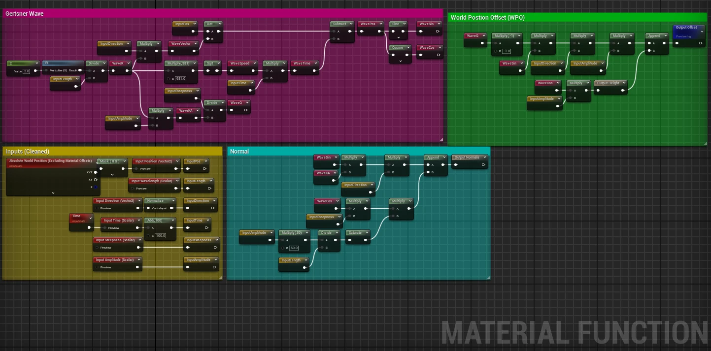
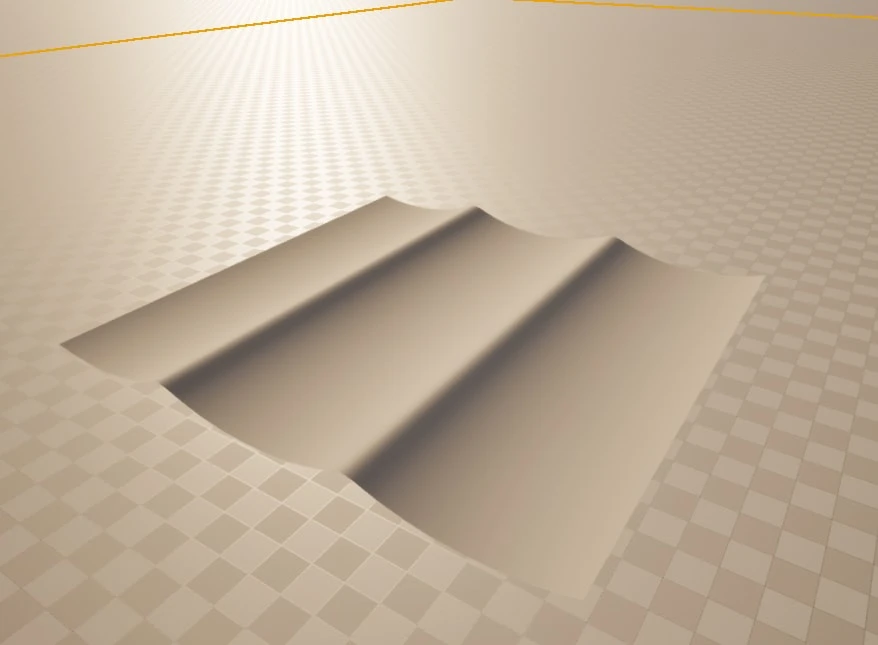
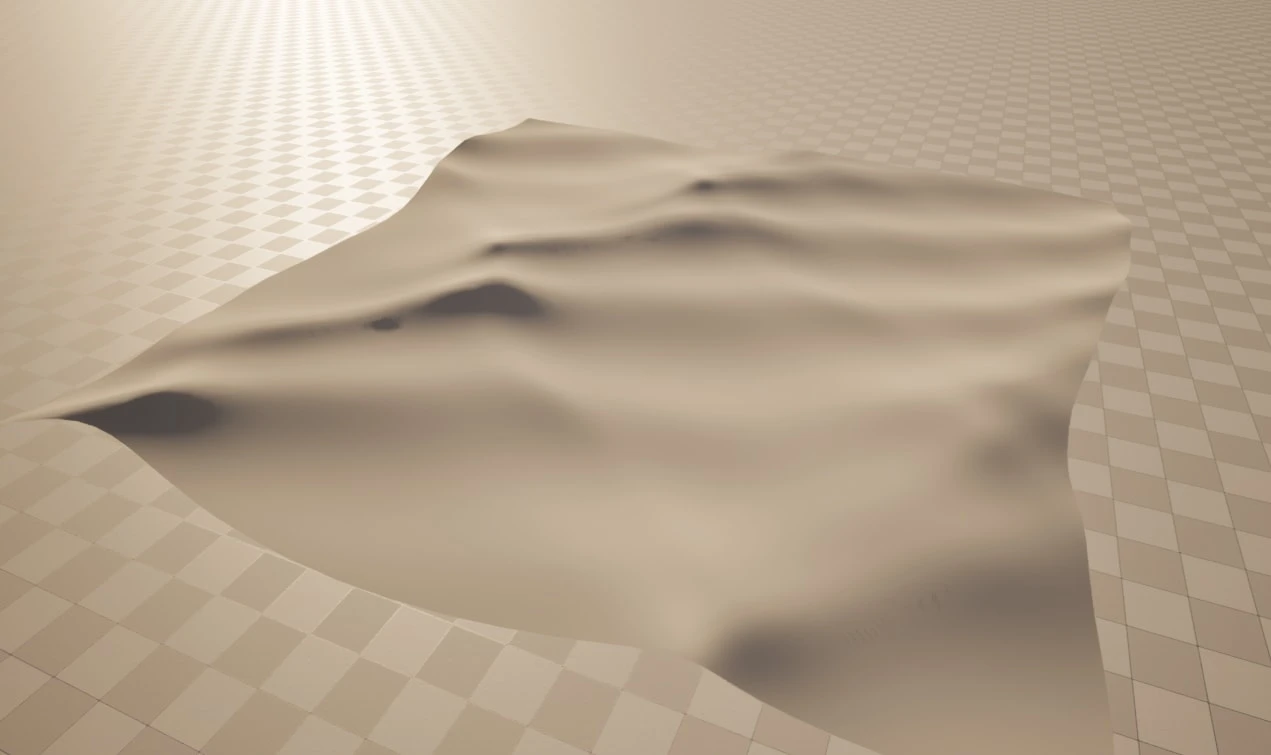
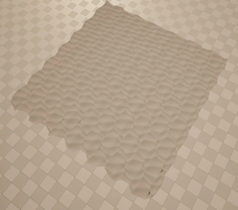
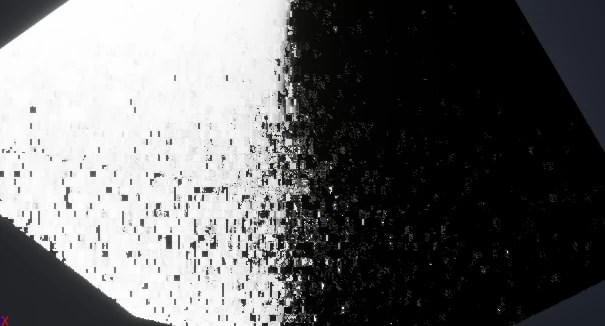
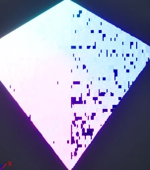
Going through these steps was highly useful, as it was a lot easier to debug when adding one aspect at a time. I used VS Code to write the HLSL and copied it into the custom node, which was much easier than trying to write it in the editor. Some of the funny bugs I encountered are shown below:

A test plane with world position offset gone wrong, erupting into a dense block of vertical spikes — Bug 1 - Wrong WPO

A test plane covered in a regular pattern of small dimples instead of a wave — Bug 2 - Incorrect wave addition

A broken render of the ocean plane, split into hard black and white blocks — Bug 3 - Unknown HLSL

A diamond shaped patch of ocean rendered in pale blue and white, scattered with blocky dark purple artefacts — Bug 4 - Another Unknown HLSL

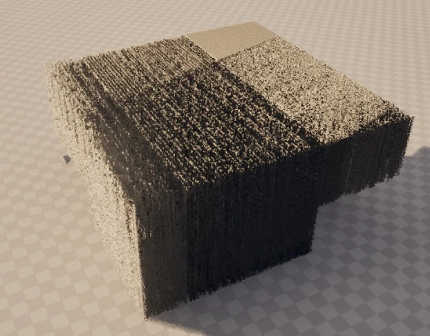
The equation

The equation is Tessendorf’s Gerstner wave from Simulating Ocean Water (Tessendorf, 2001). The one change is that the horizontal term is scaled by a steepness $Q$ instead of the amplitude, so the sharpness of the crests can be tuned separately from their height.

This change and the Unreal implementation are heavily based on Ghislain Girardot’s breakdown (Girardot, 2022), which builds on Epic Games’ implementation in the experimental Water plugin (Epic Games, 2021), with some modifications of my own.

For a beginner’s introduction to wave simulation in general, I recommend Acerola’s How Games Fake Water (Acerola, 2023) as a starting point.

Gerstner waves vs FFT waves

Tessendorf’s paper is best known for its Fast Fourier Transform (FFT) ocean, but I used the Gerstner method from earlier in the same paper.

With Gerstner waves, each wave is a simple rolling shape, and the shader works out every wave at every vertex and adds them together. An FFT ocean starts from thousands of waves of different sizes, mixed to match how real oceans behave, and uses a maths shortcut called an inverse FFT to turn them all into one height texture each frame. The mesh then reads its shape from that texture. One of the best-known AAA examples is Rare’s ocean in Sea of Thieves. Their SIGGRAPH 2018 talk (Ang et al., 2018) covers how they kept it running in real time across a range of hardware, including aspects like collisions and weather events.

The two methods scale differently in cost. Gerstner waves scale linearly, so a handful is cheap, but every extra wave adds work at every vertex. An FFT pays a higher but fixed cost each frame to update the spectrum and run the inverse transform, so it can reach far more detail than Gerstner waves for the same price.

Illustrative example - Gerstner is cheaper at low wave counts, FFT overtakes at higher wave counts.

I chose Gerstner waves mainly because of time constraints. While I could have implemented an FFT ocean, I would not have been able to spend the time making it stylised or practical to the level I wanted.

The wave loop

The custom node is one loop over every wave. Each pass works out that wave’s size, direction and phase, then adds its share to the world position offset, the normal and a mask, so displacement and lighting share the work instead of doing it twice.

Wave size

Each wave gets its parameters from its index divided by the total wave count, and that count stays fixed even when the loop stops early. The loop runs to count_limit, but the fraction always divides by count. Lowering the limit just drops waves from the end, and the waves that remain are exactly the same waves in the same places. That’s what makes the material LODs possible. If the fraction divided by the number of waves actually run, dropping from 16 waves to 8 would change every wave, and the switch between LODs would be visible. The waves that get dropped are the ones at the max end of the ranges, so the cheaper LODs lose that end rather than a random sample. The values used in the final scene are in the material’s parameter panel.

From that fraction, each wave $i$ interpolates its wavelength $L$ , steepness $Q$ and amplitude $A$ between ranges the artist sets, biased by a distribution exponent so the spread of wave sizes can be tuned instead of always being linear:

α L, Q, A = (\frac{i}{count})^{distribution} = lerp (min, max, α)

float actual_waves = min(count_limit, count);

for (int i = 0; i < actual_waves; i++)
{
    const float i_fraction = (float)i / (float)count;
    const float alpha = pow(i_fraction, distribution);

    const float length = lerp(length_range.x, length_range.y, alpha);
    const float steepness = lerp(steepness_range.x, steepness_range.y, alpha);
    const float amplitude = lerp(amplitude_range.x, amplitude_range.y, alpha);
    // ...
}

Direction

Directions come from a small pseudo-random generator seeded with two primes, then get blended towards a wind direction the artist sets, using a spread parameter. At zero spread every wave runs with the wind and the water reads as one directional swell, and turning it up makes the surface choppier and less organised. The generator is deterministic on purpose, because the same seed has to give the same ocean every time the shader compiles.

rng_x = (rng_x * 1103515245) + 12345;
rng_y = (rng_y * 1103515245) + 12345;
float2 direction = float2(cos((float)rng_x / 801571.f), sin((float)rng_y / 10223.f));
direction = normalize(lerp(wind_direction, (direction * 2.f) - 1.f, spread));

Speed and phase

Wave speed comes from the deep water dispersion relation using real gravity, so long waves travel faster than short ones, as they do in real life, without anyone having to tune it. The wavelength gives the wavenumber $k$ , that gives the angular speed $ω$ , and together they give the phase $θ$ at a point $p$ on the flat mesh, for a wave travelling in direction $D$ :

k ω θ = \frac{2 π}{L} = g k = k (D \cdot p) - ω t

float dispersion = tau / length;
float speed = sqrt(dispersion * 981.f);
float wave_time = speed * time;
float pos = dot(position, direction * dispersion) - wave_time;

Offset and normal

The offset sums every wave. The horizontal term pulls points towards each crest, which is what sharpens them, and the vertical term is the height:

offset_{x y} offset_{z} = - i \sum \frac{Q}{k} D sin θ = i \sum A cos θ

The normal is summed in the same pass, with $a = saturate (50 A)$ :

N_{x y} N_{z} N = i \sum A k D sin θ = 1 - i \sum \frac{Q a}{L} cos θ = normalize (N_{x y}, N_{z})

The normal’s vertical term is the one place mine differs from the textbook, which would use $Q k A$ . It uses a clamped amplitude over the wavelength instead, so small waves don’t flatten the normal out.

o_xy += -strength * wave_sin * direction * amplitude;
o_z += wave_cos * amplitude;
n_xy += wave_sin * intensity * direction;
n_z += wave_cos * steepness * clamped_amplitude / length;

Full HLSL

The full custom node, with the maths mapped to its variables. (HLSL, 60 lines)

Maths	In the HLSL
$α$	`alpha`, from `i_fraction`
$L, Q, A$	`length`, `steepness`, `amplitude`
$k$	`dispersion`
$ω t$	`wave_time`
$θ$	`pos`
$D$	`direction`, blended toward `wind_direction` by `spread`
$Q / k$	`strength * amplitude`, since `strength = steepness / (amplitude * k)`
$offset$	`o_xy`, `o_z`, output as `WPO`
$N$	`n_xy`, `n_z`, output as `Normal`

// WPO XYZ
float2 o_xy = float2(0.0f, 0.0f);
float o_z = 0.0f;
// Normal XYZ
float2 n_xy = float2(0.0f, 0.0f);
float n_z = 0.0f;
// Mask Z
float m_z = 0.0f;

// Start primes
int rng_x = 1000211;
int rng_y = 11587;

float actual_waves = min(count_limit, count);

// Loop through waves
for (int i = 0; i < actual_waves; i++)
{
    // Using a normalised fraction of the wave count allows waves to be consistent even at distance
    const float i_fraction = (float)i / (float)count;
    const float alpha = pow(i_fraction, distribution);

    // Computed wave param based on alpha
    const float length = lerp(length_range.x, length_range.y, alpha);
    const float steepness = lerp(steepness_range.x, steepness_range.y, alpha);
    const float amplitude = lerp(amplitude_range.x, amplitude_range.y, alpha);
    const float clamped_amplitude = saturate(amplitude * 50.f);

    // Random Direction
    rng_x = (rng_x * 1103515245) + 12345;
    rng_y = (rng_y * 1103515245) + 12345;
    float2 direction = float2(cos((float)rng_x / 801571.f), sin((float)rng_y / 10223.f));
    // User-authored direction
    direction = normalize(lerp(wind_direction, (direction * 2.f) - 1.f, spread));

    // Gerstner wave
    float tau = 2.f * PI;
    float dispersion = tau / length;
    float speed = sqrt(dispersion * 981.f);
    float wave_time = speed * time;
    float pos = dot(position, direction * dispersion) - wave_time;
    float wave_sin = sin(pos);
    float wave_cos = cos(pos);
    float intensity = amplitude * dispersion;
    float strength = steepness / intensity;

    // Result WPO
    o_xy += -strength * wave_sin * direction * amplitude;
    o_z += wave_cos * amplitude;
    // Result Normal
    n_xy += wave_sin * intensity * direction;
    n_z += wave_cos * steepness * clamped_amplitude / length;
    // Result Mask
    m_z += wave_cos / count;
}
WPO = float3(o_xy.x, o_xy.y, o_z);
Normal = normalize(float3(n_xy.x, n_xy.y, 1.f - n_z));
Mask = m_z;
Height = o_z;
return 0;

Sources

Acerola (2023). How Games Fake Water. [online] YouTube. Available at: https://www.youtube.com/watch?v=PH9q0HNBjT4 [Accessed 1 Oct. 2026].
An easy-to-follow introduction to how games fake water by summing waves.
Ang, N., Catling, A., Cifariello Ciardi, F. and Kozin, V. (2018). The Technical Art of Sea of Thieves. [online] SIGGRAPH 2018 Talks, Vancouver. Reuploaded to YouTube by iamarugin. Available at: https://www.youtube.com/watch?v=y9BOz2dFZzs [Accessed 1 Oct. 2026].
How a AAA studio handled a real-time stylised ocean with FFT waves. Video is reupload, SIGGRAPH History Archive (https://history.siggraph.org/learning/the-technical-art-of-sea-of-thieves-by-ang-catling-ciardi-and-kozin/).
Epic Games (2021). GerstnerWaveFunctions.ush, Unreal Engine Water plugin source code. [online] GitHub. Available at: https://github.com/EpicGames/UnrealEngine/blob/46544fa5e0aa9e6740c19b44b0628b72e7bbd5ce/Engine/Plugins/Experimental/Water/Shaders/Private/GerstnerWaveFunctions.ush [Accessed 1 Oct. 2026].
Epic's HLSL implementation of Gerstner waves from the experimental Water plugin.
Girardot, G. (2022). A deep dive into my process of creating this animated stylized ocean in UE. [online] YouTube. Available at: https://www.youtube.com/watch?v=UWGwq-_w08c [Accessed 1 Oct. 2026].
My main reference for building Gerstner waves.
Tessendorf, J. (2001). Simulating Ocean Water. [online] Available at: https://people.computing.clemson.edu/~jtessen/reports/papers_files/coursenotes2004.pdf [Accessed 21 Jan. 2025].
The Gerstner wave formula.